mkdifflc - An Image-Subtraction-Based Photometry Routine
Motivation: this routine was designed to extract the light curve of a SN superposed
on a non-trivial background (a clumpy host galaxy), that requires image subtraction
to minimize photometry contamination by background light. The routine extracts the
light curve (including errors) directly from a stack of fits images. This routine
will also be useful to study other variable sources superposed on non-trivial background,
such as (relatively nearby) GRBs, low-luminosity AGN, and variable stars in very crowded
fields.
Algorithm: this routine implements the algorithm described in Gal-Yam et al. (2004).
The image stack is carefully registered. One image (typically the one with least or no flux from the
transient source) is designated as the reference. A negative artificial point source, (hereafter the "artificial
reference star") is introduced into the reference image, which is then subtracted from all other images
using the PSF-matching image subtraction "Common PSF Method" (CPM, aka "Double Degradation Algorithm",
DDA, Gal-Yam, Poznanski and Maoz, in prep.). The artificial reference star appears as a positive source in all
the resulting difference images. This source is known (of course) to be constant, and has the appropriate PSF
in each difference image (the PSF of the reference image, convolved with the PSF of the image from which
it was subtracted). Since CPM removes most of the background contaminating light, we can now use aperture photometry
(with the aperture radius determined from the artificial reference star) to measure the relative photometry
of the SN with respect to the artificial constant reference star. This light curve can be set on an absolute scale by
calibrating the flux of the artificial star at any epoch. The errors are determined by placing up to 10 artificial "SNe" in locations
(interactively determined by the user) which are similar in terms of background to the location of the SN or other
transient source in question. These artificial SNe are photometered in the same way as the real SN, and the photometry
error is determined from their scatter. This error includes both Poisson errors and the additional errors introduced
by non-perfect image subtraction.
How to use mkdifflc:
The algorithm is implemented in an IRAF script mkdifflc.cl. The script has
four stages. The script requires as input the name of a file containing a list of all the relevant images, one image
name per line, which ends with a carriage return and contains no empty lines. More input parameters are described
below.
Stage one is designed to roughly align the input images, which are assumed to have the same
orientation, but may have arbitrarily large offsets. If applying this to P60 images, I like to align then
with north up and east to the left - this means flopping images from the old ccd around the X-axis, and
rotating images from the new ccd by 87.88 degrees. The actual alignment is interactively done by the user, as the
images are displayed one by one and the user is prompted to identify an object of his choice in each image
(it has to be the same object in all of them, of course, so choose a prominent star you can easily identify even
if there is a large offset). If you prefer to align your images using some other way (e.g., by their WCS) you
can go directly to stage 2. Warning: I found that using wcs registering (e.g., by the "wregister" IRAF task) on
P60 images is not good enough, as the WCS may be off by many arcseconds in some cases. But you may do better than
me (tell me about it).
Stage two uses the IRAF tasks GEOMAP and GEOTRAN to ACCURATELY register all the images to the reference (the image listed first
in the image list input by the user). The user can determine the number of sources to be used to calculate the
geometric transformation (I would use at least 10) and select them interactively (choose non-saturated, bright,
isolated stars). If you have another way to get accurate registration (to better than 0.3 pixel rms), you can
start with stage 3, and again - please tell me about it.
Stage three uses CPM to subtract the reference frame (the FIRST image in the file supplied by the user) from
all the rest. The user is interactively prompted to select the PSF stars to be used by CPM. Here, my experience is
that 3-5 stars are enough, and that bright, isolated stars only should be selected - it is better to have
a few (even one) bright good stars than a long list of stars, many of which are faint (introducing lots of
noise to the PSF) or have nearby neighbors (again contaminating the PSF). The user is also prompted to set the
flux and position of the artificial reference star.
This image shows the quality of image
subtraction you obtain by applying CPM to P60 images of SN 2004A collected with both the old and new CCD.
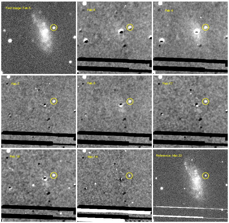
Notes: (1) In this case, the reference image does contain SN light (this is a slowly declining SN II-P). This causes
no real trouble. (2) There is no problem in subtracting a new CCD reference image (the March 23 image) from old ccd images
(those prior to March 1). (3) CPM deals very well with variable seeing, and also corrects for the P60 focus problems. Images
with effective seeing (measured FWHM, seeing + any focus offsets) better than 5" do not leave any residual galactic background.
The image from Feb 6, with effective seeing 5.5", has some marginal fuzzy residual. An image from Feb 13 (with effective
seeing ~8") had to be rejected - the PSF is probably ill-defined there (a donut). (4) The artificial reference stars
can be seen in the top right corner of the difference images.
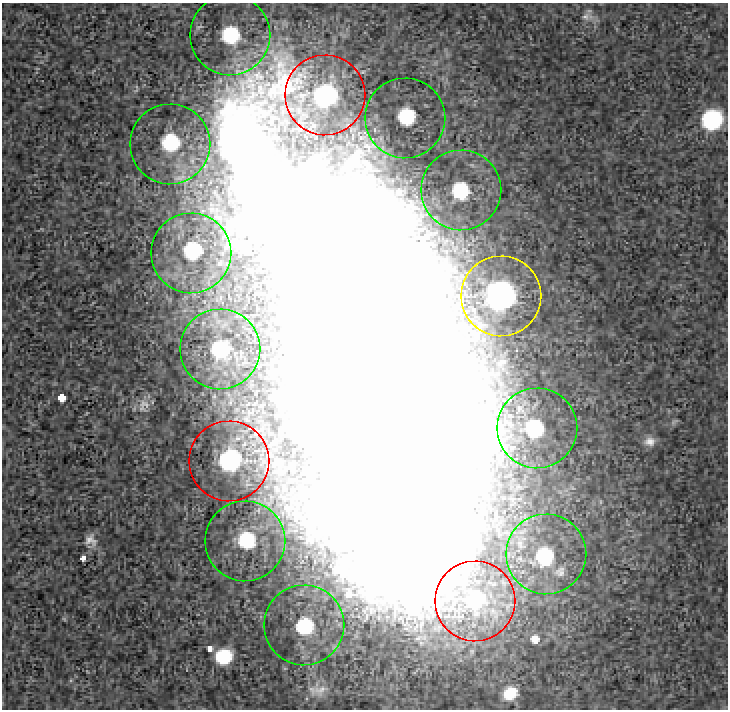
The last stage calculates the photometry and errors. The user is asked to identify the location of the SN in one of the
difference images, and to place up to 10 "fake" SNe in locations which have similar background properties. This is
done by hand since a general procedure to determine what "similar" means in a general way is impossible. For some
uses (e.g. images with many similar galaxies, say) some automated procedure may be devised. The following image
shows the host of SN 2004A (yellow) with 10 additional "fake" SNe (green). Some nearby non-variable point sources
(which happen to be around that galaxy) are also marked (red).
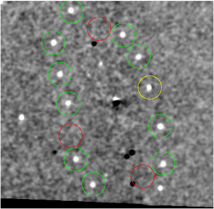
CPM is then used again, and the flux of the fake SNe is measured and compared with that of the real SN. The program then
iterates so that the mean flux of the fake SNe equals that of the real SN, to correctly account for Poisson errors.
This image shows the difference image after subtraction. Note that the real and fake SNe (yellow and green) have
the same flux, while the non-variable sources (red) are gone.
Finally, the program reads the date (JD or MJD) from the header, and
outputs the measurements into a file, one file per image. The format is as follows:
% magnitude offset from the reference artificial star, and JD/MJD:
4.04 2453078.840
% ratio of SN flux to artificial star flux, and JD/MJD:
0.024177359203342 2453078.840
% SN magnitude and flux:
18.15 550.4
% fake stars magnitudes and fluxes:
18.17 541.7
18.35 455.1
18.07 591.5
18.02 621.
18.25 502.5
18.16 545.9
18.12 566.1
18.14 553.
18.07 594.2
17.94 666.
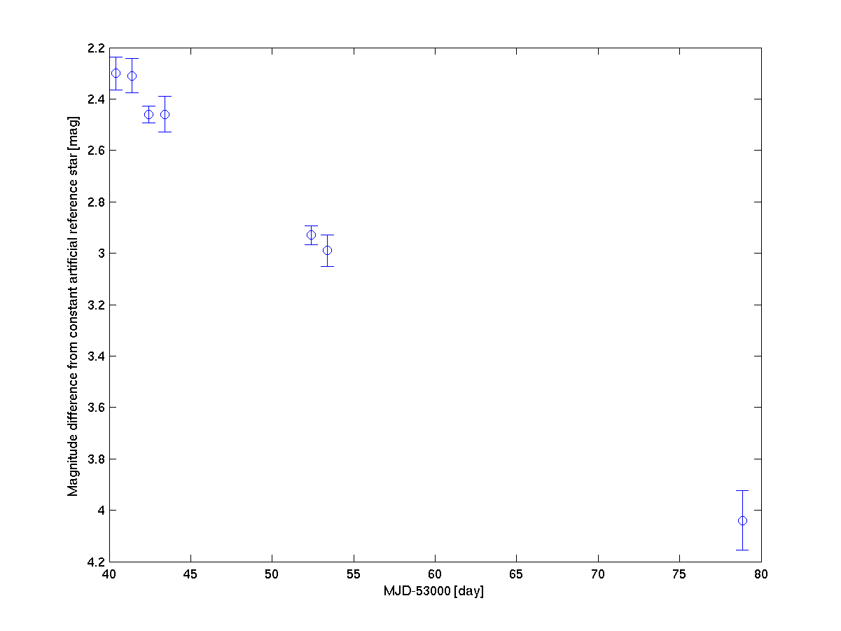
You can read these data into your favorite analysis program, get the Mag(day) or flux(day) light curves
from the upper rows, and derive the errors from the scatter of the lower rows. A short matlab
script that reads the list of output files produced by mkdifflc (called 'lclist') and generates
a light curve with errors can be found here. A light curve
derived from the exemplary data discussed above using this matlab script is shown here:
That's it for now. This routine is far from being fully-tested, but I think it can definitely be
used. I'll be glad to sit/talk with whoever wants help using these tools.
PS. The mkdifflc.cl parameter file looks like that:
(beginst= 4) The beginning step(1=shift,2=register,3=diff,4=errcalc
(imageli= imagelist) list of images
(starnum= 20) number of stars for registration
(ximsize= 2048.) image size in pixels, x
(yimsize= 2048.) image size in pixels, y
(psfsize= 21.) psf size to use in fcpmxn
(diffnum= 9) number of independent image (excluding the reference image
(lis = imagelist)
(temp = junk)
(temp1 = )
(mode = ql)
The only thing that is not self-explanatory is "psfsize" - this is the size of the
area extracted by CPM to determine the empirical PSF. I found that 21 works well for images
with FWHM 3-15 pixels. If you have extremely well sampled PSF (FWHM>15 pixels), perhaps
you should set this to a larger number, but this will increase running time of this
routine.
Constructed: May 2004, by Avishay Gal-Yam, E-Mail: avishay@astro.caltech.edu
